 Qiusheng Wu
38ed979d3b
* docs: review the docs against the code and fix drift

Check every docs page against the current code and correct what no
longer matches: menu paths and labels, plugin placement (most plugins
now open in a docked panel), Cesium ion tokens being optional, desktop
OAuth sign-in for sharing, browser project save/open, project schema
fields, server and collaboration endpoints, Python and MCP APIs, and
stale paths in the source-code deep dives.

Fix the Spatial SQL tutorial's ST_Area_Spheroid query, which needs
ST_FlipCoordinates for lat/lon axis order. Document the Settings
sections that were listed but never described (Language, Appearance,
Interface, Geocoding, AI Providers), and add the USGS NLDI and ArcGIS
feature editing pages to the nav.

* docs: keep the NLDI and ArcGIS editing pages out of the nav

* Address CodeRabbit review feedback

- collaboration.md: give both snapshot-cap defaults, 10 MB for the
  relay and 1 MB in the Docker Compose setup.
- features.md, cesium-renderer.md: without an Ion token the globe still
  gets terrain from keyless Terrarium elevation (or a configured COG),
  not a bare ellipsoid (cesium-engine.ts enableWorldTerrain).

* Address CodeRabbit review feedback

- project-format.md: type blankBackgroundColor and selectedLayerId as
  string | null, matching ProjectFile in packages/core/src/types.ts.
2.9 KiB
Spatial SQL
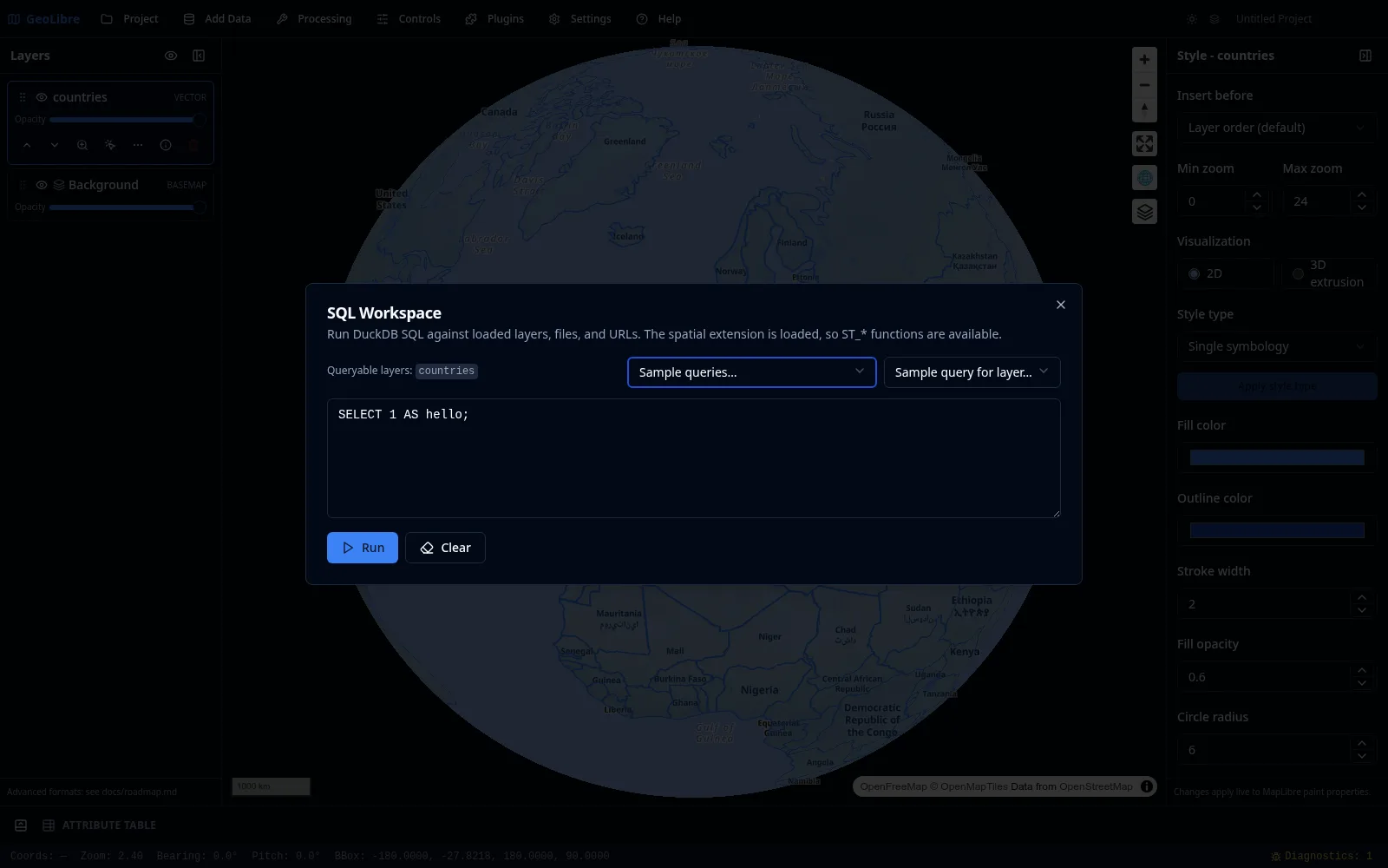
The SQL Workspace lets you analyze data with DuckDB Spatial SQL and add the results to the map. It runs on DuckDB-WASM, so it works in the browser as well as the desktop app. Open it from Processing → SQL Workspace.
1. Query a loaded layer
Every loaded vector layer is a queryable table. Load the sample countries layer (see Your First Map), then run:
SELECT NAME, CONTINENT, GDP_MD_EST
FROM countries
ORDER BY GDP_MD_EST DESC
LIMIT 10;
Click Run to see the ten countries with the highest estimated GDP.
!!! note "Sample dataset columns"
NAME, CONTINENT, POP_EST, and GDP_MD_EST are Natural Earth field names in the sample countries.parquet, whose geometry column is geom. A different dataset will have its own column names. To discover them, run DESCRIBE SELECT * FROM 'your-file-url' first.
2. Query a remote file directly
You do not have to load a file first. The Workspace detects a bare URL in a FROM clause and wraps it in the right reader automatically, then streams the file over HTTP range requests so you do not download it in full. This bare-URL shorthand is a SQL Workspace convenience; in the standard DuckDB CLI you would write read_parquet('https://...') explicitly.
SELECT COUNT(*) AS n
FROM https://data.source.coop/giswqs/opengeos/countries.parquet;
3. Use spatial functions
The spatial extension is loaded, so ST_* functions are available. For example, compute area and keep the geom column so the result can be mapped:
-- area is in square degrees because the data is in EPSG:4326;
-- the ranking is valid, but for km2 use
-- ST_Area_Spheroid(ST_FlipCoordinates(geom)) / 1e6 (it expects lat/lon order).
SELECT NAME, ST_Area(geom) AS area, geom
FROM https://data.source.coop/giswqs/opengeos/countries.parquet
WHERE CONTINENT = 'Africa'
ORDER BY area DESC;
4. Add the result to the map
When a query returns a geometry column, click Add as layer to create a new layer from the result, optionally naming it. The result layer supports identify, selection, and the attribute table like any vector layer, and you can add several result layers at once.
5. Export
Export the query result as CSV or GeoParquet straight from the workspace — the Export CSV and Export GeoParquet buttons sit beside Add as layer. See SQL Workspace.
!!! tip "Sample queries and history" Use the Sample queries… menu to start from a working query, and History… to rerun a previous one.
Next steps
- Do equivalent geometry operations with the menu-driven Vector Analysis tools.
- Convert results to cloud-native formats in Cloud-Native Data.